Fetching Evaluations

Evalutions contain a concise summary of the results of all runs made. Each evaluation provides information on the dataset used, the flow applied, the setup used, the metric evaluated, and the result obtained on the metric, for each such run made. These collection of results can be used for efficient benchmarking of an algorithm and also allow transparent reuse of results from previous experiments on similar parameters.

In this example, we shall do the following:

• Retrieve evaluations based on different metrics

• Fetch evaluations pertaining to a specific task

• Sort the obtained results in descending order of the metric

• Plot a cumulative distribution function for the evaluations

• Compare the top 10 performing flows based on the evaluation performance

import openml
from pprint import pprint

Listing evaluations

Evaluations can be retrieved from the database in the chosen output format. Required filters can be applied to retrieve results from runs as required.

# We shall retrieve a small set (only 10 entries) to test the listing function for evaluations
openml.evaluations.list_evaluations(function='predictive_accuracy', size=10,
                                    output_format='dataframe')

# Using other evaluation metrics, 'precision' in this case
evals = openml.evaluations.list_evaluations(function='precision', size=10,
                                            output_format='dataframe')

# Querying the returned results for precision above 0.98
pprint(evals[evals.value > 0.98])

Out:

     run_id  task_id  ...  values                                    array_data
62       62        1  ...    None  [0.714286,0.98,0.992658,0,0.985294,0.904762]
237     237        1  ...    None                [1,0.942857,0.991215,0,1,0.95]
413     413        1  ...    None            [1,0.980198,0.994152,0,1,0.948718]
500     500        1  ...    None         [1,0.99,0.997059,0,0.985294,0.863636]

[4 rows x 12 columns]

Viewing a sample task

Over here we shall briefly take a look at the details of the task.

# We will start by displaying a simple *supervised classification* task:
task_id = 167140        # https://www.openml.org/t/167140
task = openml.tasks.get_task(task_id)
pprint(vars(task))

Out:

{'class_labels': ['1', '2', '3'],
 'cost_matrix': None,
 'dataset_id': 40670,
 'estimation_procedure': {'data_splits_url': 'https://www.openml.org/api_splits/get/167140/Task_167140_splits.arff',
                          'parameters': {'number_folds': '10',
                                         'number_repeats': '1',
                                         'percentage': '',
                                         'stratified_sampling': 'true'},
                          'type': 'crossvalidation'},
 'estimation_procedure_id': 1,
 'evaluation_measure': None,
 'split': None,
 'target_name': 'class',
 'task_id': 167140,
 'task_type': 'Supervised Classification',
 'task_type_id': 1}

Obtaining all the evaluations for the task

We’ll now obtain all the evaluations that were uploaded for the task we displayed previously. Note that we now filter the evaluations based on another parameter ‘task’.

metric = 'predictive_accuracy'
evals = openml.evaluations.list_evaluations(function=metric, task=[task_id],
                                            output_format='dataframe')
# Displaying the first 10 rows
pprint(evals.head(n=10))
# Sorting the evaluations in decreasing order of the metric chosen
evals = evals.sort_values(by='value', ascending=False)
print("\nDisplaying head of sorted dataframe: ")
pprint(evals.head())

Out:

          run_id  task_id  setup_id  ...     value values array_data
9060101  9060101   167140   6993238  ...  0.956685   None       None
9060109  9060109   167140   6993245  ...  0.519146   None       None
9060112  9060112   167140   6993248  ...  0.964218   None       None
9060116  9060116   167140   6993252  ...  0.623666   None       None
9060117  9060117   167140   6993253  ...  0.610483   None       None
9060119  9060119   167140   6993255  ...  0.610483   None       None
9060120  9060120   167140   6993256  ...  0.610483   None       None
9060122  9060122   167140   6993258  ...  0.872567   None       None
9060127  9060127   167140   6993263  ...  0.960138   None       None
9060131  9060131   167140   6993267  ...  0.634338   None       None

[10 rows x 12 columns]

Displaying head of sorted dataframe:
            run_id  task_id  setup_id  ...     value values array_data
10228369  10228369   167140   8153634  ...  0.965160   None       None
9161834    9161834   167140   7094257  ...  0.965160   None       None
9193963    9193963   167140   7124554  ...  0.965160   None       None
9194969    9194969   167140   7125506  ...  0.965160   None       None
9198736    9198736   167140   7129205  ...  0.964846   None       None

[5 rows x 12 columns]

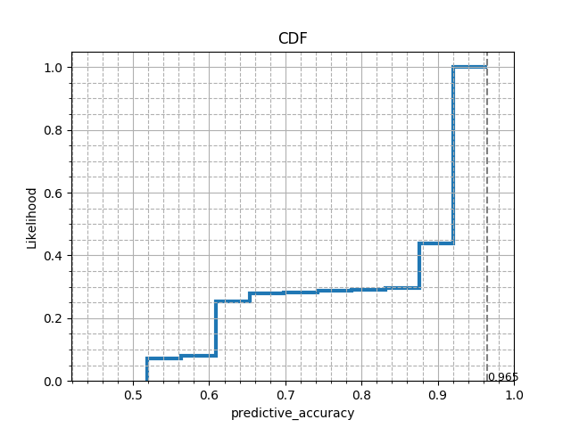
Obtaining CDF of metric for chosen task

We shall now analyse how the performance of various flows have been on this task, by seeing the likelihood of the accuracy obtained across all runs. We shall now plot a cumulative distributive function (CDF) for the accuracies obtained.

from matplotlib import pyplot as plt


def plot_cdf(values, metric='predictive_accuracy'):
    max_val = max(values)
    n, bins, patches = plt.hist(values, density=True, histtype='step',
                                cumulative=True, linewidth=3)
    patches[0].set_xy(patches[0].get_xy()[:-1])
    plt.xlim(max(0, min(values) - 0.1), 1)
    plt.title('CDF')
    plt.xlabel(metric)
    plt.ylabel('Likelihood')
    plt.grid(b=True, which='major', linestyle='-')
    plt.minorticks_on()
    plt.grid(b=True, which='minor', linestyle='--')
    plt.axvline(max_val, linestyle='--', color='gray')
    plt.text(max_val, 0, "%.3f" % max_val, fontsize=9)
    plt.show()


plot_cdf(evals.value, metric)
# This CDF plot shows that for the given task, based on the results of the
# runs uploaded, it is almost certain to achieve an accuracy above 52%, i.e.,
# with non-zero probability. While the maximum accuracy seen till now is 96.5%.

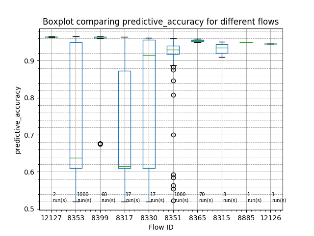
Comparing top 10 performing flows

Let us now try to see which flows generally performed the best for this task. For this, we shall compare the top performing flows.

import numpy as np
import pandas as pd


def plot_flow_compare(evaluations, top_n=10, metric='predictive_accuracy'):
    # Collecting the top 10 performing unique flow_id
    flow_ids = evaluations.flow_id.unique()[:top_n]

    df = pd.DataFrame()
    # Creating a data frame containing only the metric values of the selected flows
    #   assuming evaluations is sorted in decreasing order of metric
    for i in range(len(flow_ids)):
        flow_values = evaluations[evaluations.flow_id == flow_ids[i]].value
        df = pd.concat([df, flow_values], ignore_index=True, axis=1)
    fig, axs = plt.subplots()
    df.boxplot()
    axs.set_title('Boxplot comparing ' + metric + ' for different flows')
    axs.set_ylabel(metric)
    axs.set_xlabel('Flow ID')
    axs.set_xticklabels(flow_ids)
    axs.grid(which='major', linestyle='-', linewidth='0.5', color='gray', axis='y')
    axs.minorticks_on()
    axs.grid(which='minor', linestyle='--', linewidth='0.5', color='gray', axis='y')
    # Counting the number of entries for each flow in the data frame
    #   which gives the number of runs for each flow
    flow_freq = list(df.count(axis=0, numeric_only=True))
    for i in range(len(flow_ids)):
        axs.text(i + 1.05, np.nanmin(df.values), str(flow_freq[i]) + '\nrun(s)', fontsize=7)
    plt.show()


plot_flow_compare(evals, metric=metric, top_n=10)
# The boxplots below show how the flows perform across multiple runs on the chosen
# task. The green horizontal lines represent the median accuracy of all the runs for
# that flow (number of runs denoted at the bottom of the boxplots). The higher the
# green line, the better the flow is for the task at hand. The ordering of the flows
# are in the descending order of the higest accuracy value seen under that flow.

# Printing the corresponding flow names for the top 10 performing flow IDs
top_n = 10
flow_ids = evals.flow_id.unique()[:top_n]
flow_names = evals.flow_name.unique()[:top_n]
for i in range(top_n):
    pprint((flow_ids[i], flow_names[i]))

Out:

(12127,
 'sklearn.ensemble._hist_gradient_boosting.gradient_boosting.HistGradientBoostingClassifier(1)')
(8353,
 'sklearn.pipeline.Pipeline(imputation=hyperimp.utils.preprocessing.ConditionalImputer2,hotencoding=sklearn.preprocessing.data.OneHotEncoder,scaling=sklearn.preprocessing.data.StandardScaler,variencethreshold=sklearn.feature_selection.variance_threshold.VarianceThreshold,clf=sklearn.svm.classes.SVC)(1)')
(8399,
 'sklearn.model_selection._search.RandomizedSearchCV(estimator=sklearn.pipeline.Pipeline(imputation=hyperimp.utils.preprocessing.ConditionalImputer,hotencoding=sklearn.preprocessing.data.OneHotEncoder,scaling=sklearn.preprocessing.data.StandardScaler,variencethreshold=sklearn.feature_selection.variance_threshold.VarianceThreshold,clf=sklearn.svm.classes.SVC))(1)')
(8317,
 'sklearn.pipeline.Pipeline(imputation=hyperimp.utils.preprocessing.ConditionalImputer,hotencoding=sklearn.preprocessing.data.OneHotEncoder,scaling=sklearn.preprocessing.data.StandardScaler,variencethreshold=sklearn.feature_selection.variance_threshold.VarianceThreshold,clf=sklearn.svm.classes.SVC)(1)')
(8330,
 'sklearn.pipeline.Pipeline(imputation=openmlstudy14.preprocessing.ConditionalImputer,hotencoding=sklearn.preprocessing.data.OneHotEncoder,scaling=sklearn.preprocessing.data.StandardScaler,variencethreshold=sklearn.feature_selection.variance_threshold.VarianceThreshold,classifier=sklearn.svm.classes.SVC)(2)')
(8351,
 'sklearn.pipeline.Pipeline(imputation=hyperimp.utils.preprocessing.ConditionalImputer2,hotencoding=sklearn.preprocessing.data.OneHotEncoder,variencethreshold=sklearn.feature_selection.variance_threshold.VarianceThreshold,clf=sklearn.ensemble.forest.RandomForestClassifier)(1)')
(8365,
 'sklearn.model_selection._search.RandomizedSearchCV(estimator=sklearn.pipeline.Pipeline(imputation=hyperimp.utils.preprocessing.ConditionalImputer,hotencoding=sklearn.preprocessing.data.OneHotEncoder,variencethreshold=sklearn.feature_selection.variance_threshold.VarianceThreshold,clf=sklearn.ensemble.forest.RandomForestClassifier))(1)')
(8315,
 'sklearn.pipeline.Pipeline(imputation=hyperimp.utils.preprocessing.ConditionalImputer,hotencoding=sklearn.preprocessing.data.OneHotEncoder,variencethreshold=sklearn.feature_selection.variance_threshold.VarianceThreshold,clf=sklearn.ensemble.forest.RandomForestClassifier)(1)')
(8885,
 'sklearn.pipeline.Pipeline(imputation=preprocessing.ConditionalImputer2,catencoding=preprocessing.MultiLabelEncoder,variencethreshold=sklearn.feature_selection.variance_threshold.VarianceThreshold,clf=sklearn.ensemble.forest.RandomForestClassifier)(1)')
(12126, 'sklearn.linear_model.logistic.LogisticRegression(25)')