
Note
Go to the end to download the full example code.
Fetching Evaluations
Evaluations contain a concise summary of the results of all runs made. Each evaluation provides information on the dataset used, the flow applied, the setup used, the metric evaluated, and the result obtained on the metric, for each such run made. These collection of results can be used for efficient benchmarking of an algorithm and also allow transparent reuse of results from previous experiments on similar parameters.
In this example, we shall do the following:
Retrieve evaluations based on different metrics
Fetch evaluations pertaining to a specific task
Sort the obtained results in descending order of the metric
Plot a cumulative distribution function for the evaluations
Compare the top 10 performing flows based on the evaluation performance
Retrieve evaluations with hyperparameter settings
# License: BSD 3-Clause

import openml
Listing evaluations
Evaluations can be retrieved from the database in the chosen output format. Required filters can be applied to retrieve results from runs as required.
# We shall retrieve a small set (only 10 entries) to test the listing function for evaluations
openml.evaluations.list_evaluations(
    function="predictive_accuracy", size=10, output_format="dataframe"
)

# Using other evaluation metrics, 'precision' in this case
evals = openml.evaluations.list_evaluations(
    function="precision", size=10, output_format="dataframe"
)

# Querying the returned results for precision above 0.98
print(evals[evals.value > 0.98])
   run_id  task_id  ...  values                                    array_data
0      62        1  ...    None  [0.714286,0.98,0.992658,0,0.985294,0.904762]
1     237        1  ...    None                [1,0.942857,0.991215,0,1,0.95]
3     413        1  ...    None            [1,0.980198,0.994152,0,1,0.948718]
4     500        1  ...    None         [1,0.99,0.997059,0,0.985294,0.863636]

[4 rows x 14 columns]
Viewing a sample task
Over here we shall briefly take a look at the details of the task.
# We will start by displaying a simple *supervised classification* task:
task_id = 167140  # https://www.openml.org/t/167140
task = openml.tasks.get_task(task_id)
print(task)
OpenML Classification Task
==========================
Task Type Description: https://www.openml.org/tt/TaskType.SUPERVISED_CLASSIFICATION
Task ID..............: 167140
Task URL.............: https://www.openml.org/t/167140
Estimation Procedure.: crossvalidation
Target Feature.......: class
# of Classes.........: 3
Cost Matrix..........: Available
Obtaining all the evaluations for the task
We’ll now obtain all the evaluations that were uploaded for the task we displayed previously. Note that we now filter the evaluations based on another parameter ‘task’.
metric = "predictive_accuracy"
evals = openml.evaluations.list_evaluations(
    function=metric, tasks=[task_id], output_format="dataframe"
)
# Displaying the first 10 rows
print(evals.head(n=10))
# Sorting the evaluations in decreasing order of the metric chosen
evals = evals.sort_values(by="value", ascending=False)
print("\nDisplaying head of sorted dataframe: ")
print(evals.head())
    run_id  task_id  setup_id  ...     value values  array_data
0  9199772   167140   7130140  ...  0.938481   None        None
1  9199845   167140   7130139  ...  0.623352   None        None
2  9202086   167140   7131884  ...  0.918393   None        None
3  9202092   167140   7131890  ...  0.962335   None        None
4  9202096   167140   7131894  ...  0.961707   None        None
5  9202099   167140   7131897  ...  0.519146   None        None
6  9202125   167140   7131923  ...  0.957313   None        None
7  9202139   167140   7131937  ...  0.519146   None        None
8  9202159   167140   7131957  ...  0.628060   None        None
9  9202254   167140   7132052  ...  0.610483   None        None

[10 rows x 14 columns]

Displaying head of sorted dataframe:
        run_id  task_id  setup_id  ...     value values  array_data
2788  10279797   167140   8166877  ...  0.968613   None        None
2789  10279798   167140   8166877  ...  0.968613   None        None
2246  10232158   167140   8157180  ...  0.967671   None        None
2263  10232987   167140   8157961  ...  0.967671   None        None
2314  10271558   167140   8154506  ...  0.967043   None        None

[5 rows x 14 columns]
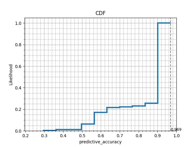
Obtaining CDF of metric for chosen task
We shall now analyse how the performance of various flows have been on this task, by seeing the likelihood of the accuracy obtained across all runs. We shall now plot a cumulative distributive function (CDF) for the accuracies obtained.
from matplotlib import pyplot as plt


def plot_cdf(values, metric="predictive_accuracy"):
    max_val = max(values)
    n, bins, patches = plt.hist(values, density=True, histtype="step", cumulative=True, linewidth=3)
    patches[0].set_xy(patches[0].get_xy()[:-1])
    plt.xlim(max(0, min(values) - 0.1), 1)
    plt.title("CDF")
    plt.xlabel(metric)
    plt.ylabel("Likelihood")
    plt.grid(visible=True, which="major", linestyle="-")
    plt.minorticks_on()
    plt.grid(visible=True, which="minor", linestyle="--")
    plt.axvline(max_val, linestyle="--", color="gray")
    plt.text(max_val, 0, "%.3f" % max_val, fontsize=9)
    plt.show()


plot_cdf(evals.value, metric)
# This CDF plot shows that for the given task, based on the results of the
# runs uploaded, it is almost certain to achieve an accuracy above 52%, i.e.,
# with non-zero probability. While the maximum accuracy seen till now is 96.5%.
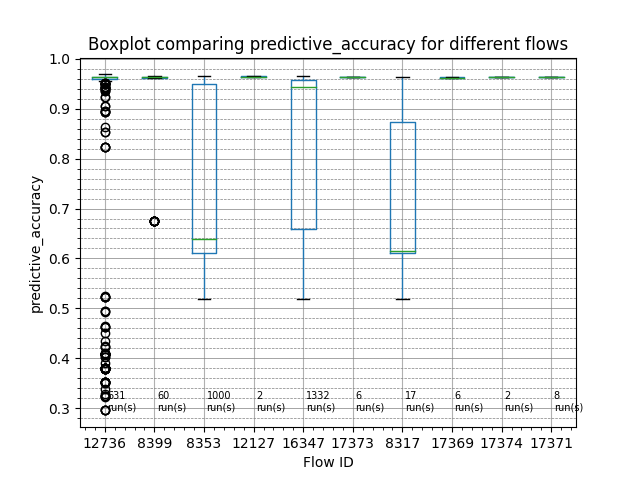
Comparing top 10 performing flows
Let us now try to see which flows generally performed the best for this task. For this, we shall compare the top performing flows.
import numpy as np
import pandas as pd


def plot_flow_compare(evaluations, top_n=10, metric="predictive_accuracy"):
    # Collecting the top 10 performing unique flow_id
    flow_ids = evaluations.flow_id.unique()[:top_n]

    df = pd.DataFrame()
    # Creating a data frame containing only the metric values of the selected flows
    #   assuming evaluations is sorted in decreasing order of metric
    for i in range(len(flow_ids)):
        flow_values = evaluations[evaluations.flow_id == flow_ids[i]].value
        df = pd.concat([df, flow_values], ignore_index=True, axis=1)
    fig, axs = plt.subplots()
    df.boxplot()
    axs.set_title("Boxplot comparing " + metric + " for different flows")
    axs.set_ylabel(metric)
    axs.set_xlabel("Flow ID")
    axs.set_xticklabels(flow_ids)
    axs.grid(which="major", linestyle="-", linewidth="0.5", color="gray", axis="y")
    axs.minorticks_on()
    axs.grid(which="minor", linestyle="--", linewidth="0.5", color="gray", axis="y")
    # Counting the number of entries for each flow in the data frame
    #   which gives the number of runs for each flow
    flow_freq = list(df.count(axis=0, numeric_only=True))
    for i in range(len(flow_ids)):
        axs.text(i + 1.05, np.nanmin(df.values), str(flow_freq[i]) + "\nrun(s)", fontsize=7)
    plt.show()


plot_flow_compare(evals, metric=metric, top_n=10)
# The boxplots below show how the flows perform across multiple runs on the chosen
# task. The green horizontal lines represent the median accuracy of all the runs for
# that flow (number of runs denoted at the bottom of the boxplots). The higher the
# green line, the better the flow is for the task at hand. The ordering of the flows
# are in the descending order of the higest accuracy value seen under that flow.

# Printing the corresponding flow names for the top 10 performing flow IDs
top_n = 10
flow_ids = evals.flow_id.unique()[:top_n]
flow_names = evals.flow_name.unique()[:top_n]
for i in range(top_n):
    print((flow_ids[i], flow_names[i]))
(12736, 'sklearn.pipeline.Pipeline(simpleimputer=sklearn.impute._base.SimpleImputer,histgradientboostingclassifier=sklearn.ensemble._hist_gradient_boosting.gradient_boosting.HistGradientBoostingClassifier)(1)')
(8399, 'sklearn.model_selection._search.RandomizedSearchCV(estimator=sklearn.pipeline.Pipeline(imputation=hyperimp.utils.preprocessing.ConditionalImputer,hotencoding=sklearn.preprocessing.data.OneHotEncoder,scaling=sklearn.preprocessing.data.StandardScaler,variencethreshold=sklearn.feature_selection.variance_threshold.VarianceThreshold,clf=sklearn.svm.classes.SVC))(1)')
(8353, 'sklearn.pipeline.Pipeline(imputation=hyperimp.utils.preprocessing.ConditionalImputer2,hotencoding=sklearn.preprocessing.data.OneHotEncoder,scaling=sklearn.preprocessing.data.StandardScaler,variencethreshold=sklearn.feature_selection.variance_threshold.VarianceThreshold,clf=sklearn.svm.classes.SVC)(1)')
(12127, 'sklearn.ensemble._hist_gradient_boosting.gradient_boosting.HistGradientBoostingClassifier(1)')
(16347, 'sklearn.pipeline.Pipeline(simpleimputer=sklearn.impute._base.SimpleImputer,onehotencoder=sklearn.preprocessing._encoders.OneHotEncoder,svc=sklearn.svm.classes.SVC)(1)')
(17373, 'sklearn.model_selection._search_successive_halving.HalvingRandomSearchCV(estimator=sklearn.ensemble._hist_gradient_boosting.gradient_boosting.HistGradientBoostingClassifier)(4)')
(8317, 'sklearn.pipeline.Pipeline(imputation=hyperimp.utils.preprocessing.ConditionalImputer,hotencoding=sklearn.preprocessing.data.OneHotEncoder,scaling=sklearn.preprocessing.data.StandardScaler,variencethreshold=sklearn.feature_selection.variance_threshold.VarianceThreshold,clf=sklearn.svm.classes.SVC)(1)')
(17369, 'sklearn.model_selection._search_successive_halving.HalvingRandomSearchCV(estimator=sklearn.ensemble._hist_gradient_boosting.gradient_boosting.HistGradientBoostingClassifier)(3)')
(17374, 'sklearn.model_selection._search.RandomizedSearchCV(estimator=sklearn.ensemble._hist_gradient_boosting.gradient_boosting.HistGradientBoostingClassifier)(4)')
(17371, 'sklearn.model_selection._search.RandomizedSearchCV(estimator=sklearn.ensemble._hist_gradient_boosting.gradient_boosting.HistGradientBoostingClassifier)(3)')
Obtaining evaluations with hyperparameter settings
We’ll now obtain the evaluations of a task and a flow with the hyperparameters
# List evaluations in descending order based on predictive_accuracy with
# hyperparameters
evals_setups = openml.evaluations.list_evaluations_setups(
    function="predictive_accuracy", tasks=[31], size=100, sort_order="desc"
)

""
print(evals_setups.head())

""
# Return evaluations for flow_id in descending order based on predictive_accuracy
# with hyperparameters. parameters_in_separate_columns returns parameters in
# separate columns
evals_setups = openml.evaluations.list_evaluations_setups(
    function="predictive_accuracy", flows=[6767], size=100, parameters_in_separate_columns=True
)

""
print(evals_setups.head(10))

""
    run_id  ...                                         parameters
0  6725054  ...  {'mlr.classif.ranger(13)_num.trees': '48', 'ml...
1  2083190  ...  {'sklearn.ensemble.forest.RandomForestClassifi...
2  3962979  ...  {'mlr.classif.ranger(13)_num.trees': '42', 'ml...
3  2083596  ...  {'sklearn.ensemble.forest.RandomForestClassifi...
4  6162649  ...  {'mlr.classif.ranger(13)_num.trees': '715', 'm...

[5 rows x 15 columns]
    run_id  ...  mlr.classif.xgboost(9)_nthread
0  2420531  ...                             NaN
1  2420532  ...                             NaN
2  2420533  ...                             NaN
3  2420534  ...                             NaN
4  2420535  ...                             NaN
5  2420536  ...                             NaN
6  2420537  ...                             NaN
7  2431903  ...                             NaN
8  2432142  ...                             NaN
9  2432377  ...                             NaN

[10 rows x 29 columns]

''
Total running time of the script: (0 minutes 15.472 seconds)