Strang et al. (2018)

A tutorial on how to reproduce the analysis conducted for Don’t Rule Out Simple Models Prematurely: A Large Scale Benchmark Comparing Linear and Non-linear Classifiers in OpenML.

Publication

Don’t Rule Out Simple Models Prematurely: A Large Scale Benchmark Comparing Linear and Non-linear Classifiers in OpenML

Benjamin Strang, Peter van der Putten, Jan N. van Rijn and Frank Hutter

In Advances in Intelligent Data Analysis XVII 17th International Symposium, 2018

Available at https://link.springer.com/chapter/10.1007%2F978-3-030-01768-2_25

# License: BSD 3-Clause

import matplotlib.pyplot as plt
import openml
import pandas as pd

A basic step for each data-mining or machine learning task is to determine which model to choose based on the problem and the data at hand. In this work we investigate when non-linear classifiers outperform linear classifiers by means of a large scale experiment.

The paper is accompanied with a study object, containing all relevant tasks and runs (study_id=123). The paper features three experiment classes: Support Vector Machines (SVM), Neural Networks (NN) and Decision Trees (DT). This example demonstrates how to reproduce the plots, comparing two classifiers given the OpenML flow ids. Note that this allows us to reproduce the SVM and NN experiment, but not the DT experiment, as this requires a bit more effort to distinguish the same flow with different hyperparameter values.

study_id = 123
# for comparing svms: flow_ids = [7754, 7756]
# for comparing nns: flow_ids = [7722, 7729]
# for comparing dts: flow_ids = [7725], differentiate on hyper-parameter value
classifier_family = "SVM"
flow_ids = [7754, 7756]
measure = "predictive_accuracy"
meta_features = ["NumberOfInstances", "NumberOfFeatures"]
class_values = ["non-linear better", "linear better", "equal"]

# Downloads all evaluation records related to this study
evaluations = openml.evaluations.list_evaluations(
    measure, size=None, flows=flow_ids, study=study_id, output_format="dataframe"
)
# gives us a table with columns data_id, flow1_value, flow2_value
evaluations = evaluations.pivot(index="data_id", columns="flow_id", values="value").dropna()
# downloads all data qualities (for scatter plot)
data_qualities = openml.datasets.list_datasets(
    data_id=list(evaluations.index.values), output_format="dataframe"
)
# removes irrelevant data qualities
data_qualities = data_qualities[meta_features]
# makes a join between evaluation table and data qualities table,
# now we have columns data_id, flow1_value, flow2_value, meta_feature_1,
# meta_feature_2
evaluations = evaluations.join(data_qualities, how="inner")

# adds column that indicates the difference between the two classifiers
evaluations["diff"] = evaluations[flow_ids[0]] - evaluations[flow_ids[1]]

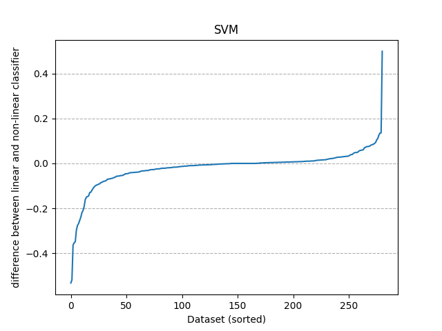
makes the s-plot

fig_splot, ax_splot = plt.subplots()
ax_splot.plot(range(len(evaluations)), sorted(evaluations["diff"]))
ax_splot.set_title(classifier_family)
ax_splot.set_xlabel("Dataset (sorted)")
ax_splot.set_ylabel("difference between linear and non-linear classifier")
ax_splot.grid(linestyle="--", axis="y")
plt.show()

adds column that indicates the difference between the two classifiers, needed for the scatter plot

def determine_class(val_lin, val_nonlin):
    if val_lin < val_nonlin:
        return class_values[0]
    elif val_nonlin < val_lin:
        return class_values[1]
    else:
        return class_values[2]


evaluations["class"] = evaluations.apply(
    lambda row: determine_class(row[flow_ids[0]], row[flow_ids[1]]), axis=1
)

# does the plotting and formatting
fig_scatter, ax_scatter = plt.subplots()
for class_val in class_values:
    df_class = evaluations[evaluations["class"] == class_val]
    plt.scatter(df_class[meta_features[0]], df_class[meta_features[1]], label=class_val)
ax_scatter.set_title(classifier_family)
ax_scatter.set_xlabel(meta_features[0])
ax_scatter.set_ylabel(meta_features[1])
ax_scatter.legend()
ax_scatter.set_xscale("log")
ax_scatter.set_yscale("log")
plt.show()

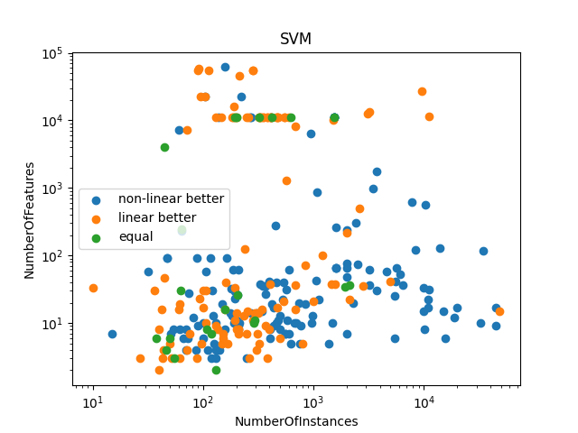
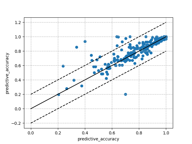
makes a scatter plot where each data point represents the performance of the two algorithms on various axis (not in the paper)

fig_diagplot, ax_diagplot = plt.subplots()
ax_diagplot.grid(linestyle="--")
ax_diagplot.plot([0, 1], ls="-", color="black")
ax_diagplot.plot([0.2, 1.2], ls="--", color="black")
ax_diagplot.plot([-0.2, 0.8], ls="--", color="black")
ax_diagplot.scatter(evaluations[flow_ids[0]], evaluations[flow_ids[1]])
ax_diagplot.set_xlabel(measure)
ax_diagplot.set_ylabel(measure)
plt.show()